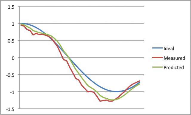
In the context of AR and VR systems, predictive tracking refers to the process of predicting the future orientation and/or position of an object or body part. For instance, one might want to predict the orientation of the head or the position of the hand.
Yuval is CEO of Sensics and co-founder of OSVR. Yuval and his team designed the OSVR software platform and built key parts of the OSVR offering. He frequently shares his views and knowledge on his blog.
Why Predictive Tracking is Useful
One common use of predictive tracking is to reduce the apparent ‘motion-to-photon’ latency, meaning the time between movement and when that movement is reflected on the display. Since there is some delay between the movement itself and when the information about that movement ends up on the screen (more on the sources of that delay below), using an estimated future orientation and position as the data used in updating the display could shorten the perceived latency.
While a lot of attention has been focused on predictive tracking in virtual reality applications, it is also very important in augmented reality, especially because the viewer has the instantaneous movement of the real world to compare against the augmented reality overlay. For instance, if you are displaying a graphical overlay to appear on top of a physical object that you see with an augmented reality headset, it is important that the overlay stays ‘locked’ to the object even when you rotate your head so that it appears to be part of the real world. The object might be recognized with a camera, but it takes time for the camera to capture the frame, for a processor to determine where the object is in the frame and for a graphics chip to render the new location of the overlay. By using predictive tracking, you can potentially reduce the movement of the overlay compared to the real world.
How Predictive Tracking Works
 If you saw a car travelling at a constant speed and you wanted to predict where that car will be one second in the future, you could probably make a fairly accurate prediction. You know the current position of the car, you might know (or can estimate) the current velocity, and thus you can extrapolate the position into the near future.
Of course if you compare your prediction with where the car actually is in one second, your prediction is unlikely to be 100% accurate every time: the car might change direction or speed up during that time. The farther out you are trying to predict, the less accurate your prediction will be: predicting where the car will be in one second is likely much more accurate than predicting where it will be in one minute.
The more you know about the car and its behavior, the better chance you have of making an accurate prediction. For instance, if you were able to measure not only the velocity but also the acceleration, you can make a more accurate prediction.
If you have additional information about the behavior of the tracked body, this can also improve prediction accuracy. For instance, when doing head-tracking, understand how fast the human head can possibly rotate and the common rotation speeds are, can improve the tracking model. Similarly, if you are doing eye-tracking, you can use the eye-tracking information to anticipate head (discussed later in this post).
Sources of Latency

The desired to perform predictive tracking comes from having some latency between actual movement and how long until an image that reflects that movement can be shown on the display. Latency can come from multiple sources, such as:
- Sensing delays. The sensors (e.g. gyroscope) may be bandwidth-limited and do not instantaneously report orientation or position changes. Similarly, camera-based sensors may exhibit delay between when the pixel on the camera sensor receives light from the tracked object and when that frame is ready to be sent to the host processor.
- Processing delays. Sensor data is often combined using some kind of sensor-fusion algorithm, and executing this algorithm can add latency between when the data is received and when the algorithm outputs the answer.
- Data smoothing. Sensor data is sometimes noisy and to avoid erroneous jitter, software or hardware-based low-pass algorithms are executed.
- Transmission delays. For example, if orientation sensing is done using a USB-connected device, there is some time between data collection by the host processor and the time data transferred over USB.
- Rendering delays. When rendering a complex scene takes some time for the processor to decide where to place every pixel on a frame and when that frame is ready to be sent to the display.
- Frame rate delays. If a display is operating at 100Hz, for instance, there is a 10 mSec time from one frame to the next. Information that is not precisely current to when a particular pixel is drawn may need to wait until the next time that pixel is drawn on the display.
Some of these delays are very small, but unfortunately all of them add up; predictive tracking, along with other techniques such as time-warping, are helpful in reducing the apparent latency.
How Far to Predict into the Future?
In two words: it depends. You will want to estimate the end-the-end latency of your system as a starting point and then optimize the timing to your liking.
It may be that you will need to predict several timepoints into the future at any given time. Here are some examples why this may be required:
- There are objects with different end-to-end delays. For instance, a hand tracked with a camera may be have different latency than a head tracker, but both need to be drawn in sync in the same scene, so predictive tracking with different ‘look ahead’ times will be used.
- In configurations where a single screen—such as a smartphone screen—is used to provide imagery to both eyes, it is often the case that the image for one eye appears with a delay of half a frame (e.g. half of 1/60 seconds, or approx 8 mSec) relative to the other eye. In this case, it is best to use predictive tracking that looks ahead 8 mSec more for that delayed half of the screen.
Common Prediction Algorithms
Here is some sampling of predictive tracking algorithms:
- Dead reckoning. This is a very simple algorithm: if the position and velocity (or angular position and angular velocity) is known at a given time, the predicted position assumes that the last know position and velocity are correct and the velocity remains the same. For instance, if the last known position is 100 units and the last known velocity is 10 units/sec, then the predicted position 10 mSec into the future is 100 + 10 x 0.01 = 100.1. While this is very simple to compute, it assumes that the last position and velocity are accurate (e.g. not subject to any measurement noise) and that the velocity is constant. Both these assumptions are often incorrect.
- Kalman predictor. This is based on a popular Kalman filter that is used to reduce sensor noise in systems where there exists a mathematical model of the system’s operation. See here for more detailed explanation of the Kalman filter.
- Alpha-beta-gamma. The ABG predictor is closely related to the Kalman predictor, but is less general and has simpler math. ABG tries to continuously estimate both velocity and acceleration and use them in prediction. Because the estimates take into account actual data, they provide some measurement noise reduction. Configuring the parameters (alpha, beta, and gamma) provide the ability to emphasize responsiveness as opposed to noise reduction.
– – — – –
Predictive tracking is a useful and commonly-used technique for reducing apparent latency. It offers simple or sophisticated implementations, requires some thought and analysis, but is essential to achieving a low latency tracking in today’s VR and AR systems.


